Predicting tumor size growth or shrinkage using ML

Scientific Machine Learning for Cancer biology

In this article, let us build a simple ML model for predicting the growth or death of a cancerous tumor. We wish to generate a forecast plot like this at the end. Let us learn how to do this.

Cancer tumor: What is it?

In our body, one rogue, mutated cell starts growing and multiplying fast. When this happens at a rapid speed, these cells accumulate to form what we know as a tumor.

Just like normal cells, cancerous cells also need space, nutrients and oxygen to grow. So the availability or limitation of either of these limits the growth of these cells and therefore the size of the tumor.

Gompertzian model for tumor growth

For phenomenon where initial rate of change is fast and later is slow, Benjamin Gomperz, a 19th century self-educated English mathematician, proposed a simple mathematical model. This model can also be used to represent the growth of cancer tumors called as the Gompertz model. It is a simple Ordinary Differential Equation (ODE).

T(t): Represents the size of the tumor at time t

r: Tumor Growth Rate. Represents how fast the tumor grows when it is small.

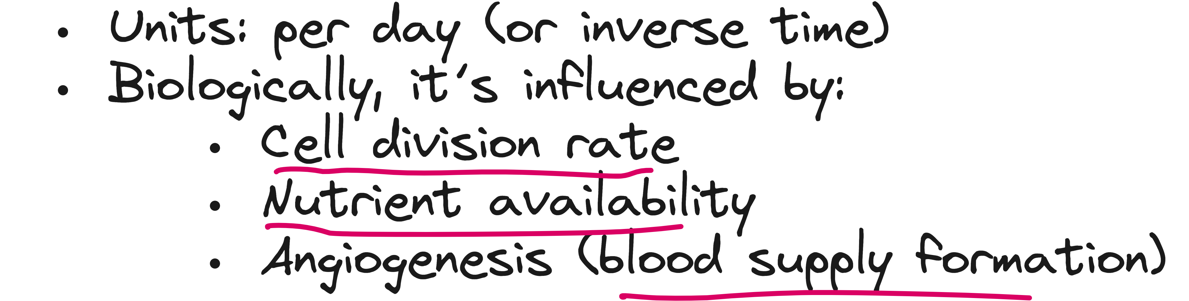
K: Carrying Capacity -- the maximum tumor size sustainable by the environment

c(t): Chemotherapy-induced kill rate.

Problem with Gompertzian model

Gompertz model is simple, but the parameters r and K are difficult to estimate in real life. C(t) may or may not be know depending on the nature of intervention (chemotherapy). Apart from being simple, the biggest problem with the Gompertz model is the empirical nature of r and K.

So what can we do here? Maybe use Machine Learning to make predictions?

What traditional ML does

If you wish to train a traditional neural network based ML model to solve this problem, instead of Gompertz model, you can do that.

Perhaps the initial value of T and the chemotherapy parameter (C) value can be the inputs to a neural network that can be trained to predict T(t=30 days).

But the problem is that you have no idea what is happening inside this model. It is literally like a blackbox. You can’t interpret the model.

Problem with traditional ML

Apart from being a blackbox, when you use a traditional ML model, you are throwing the entire framework of Gompertz into the basket.

Agreed, Gompertz model is oversimplified and the parameters r and K are difficult to estimate. But the nature of relationship between r, K and T and also the influence of chemotherapy on tumor growth rate can still be estimated really well using Gompertz model. So why should we throw all this knowledge into the basket and embrace a blackbox model?

Enter Scientific ML

This is where SciML enters the picture. In SciML, you don’t throw away the entire ODE. Instead you replace the unknown parameters using a neural network.

Here we leverage the "science" of tumor growth and "power" of ML.

This combination of differential equations and neural networks are called Universal Differential Equations. Why the term “universal”? Because neural networks are universal function approximators.

UDE for Gompertzian tumor growth model

We can rewrite the Gompertz ODE as a UDE by replacing r and K as the output of two separate neural networks.

But there are 2 questions.

1. What is the input to these neural networks?

2. How do we find T using UDE?

UDE neural networks

In this UDE, the input to both NN1 and NN2 are T(t). But here is the question. We don’t know T(t). Our whole idea is to predict T(t) right? Yest.

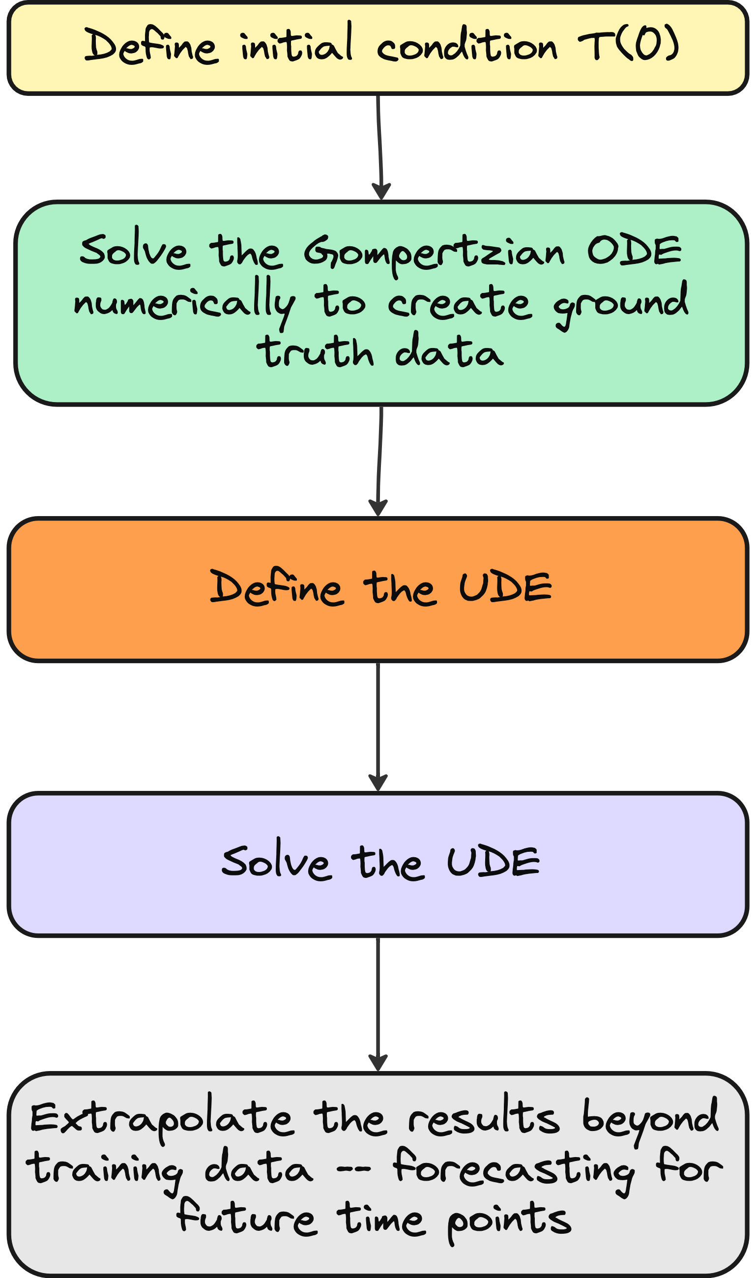
So here is what you do. You know the initial condition T(0) - the initial tumor size.

Use T(0) as the input to NN1 and NN2 to predict r and K respectively.

Now plug this predicted r and K into the Gompertz ODE to get UDE predicted dT/dt.

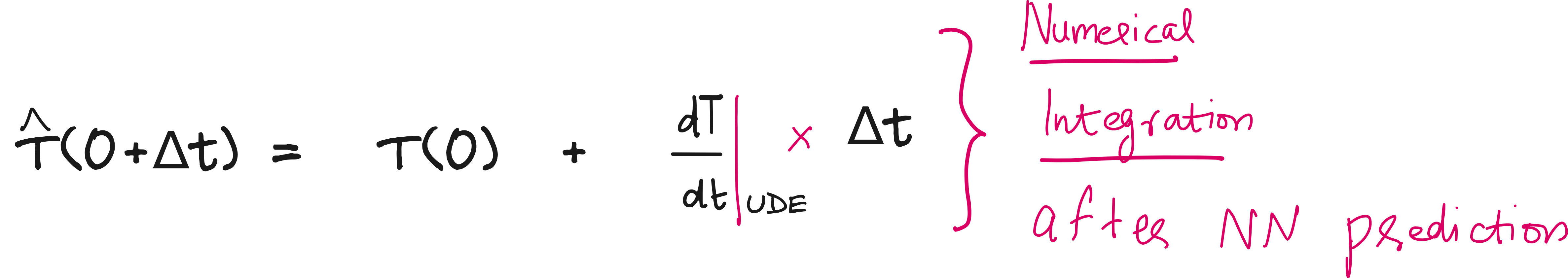
Numerical integration

Now to get the predicted T(t), you can numerically integrate the predicted dT/dt. For this, you can use Runge-Kutta numerical integration or the good old Euler integration as shown below.

Now how do you know if your predicted T is good or not? This is where the ground truth and loss function enters the picture.

Ground truth and loss function

In reality the ground truth data is obtained from actual physical experiments like MRI scan of the tumor to estimate its mass or volume. But in the absence of that you can numerically solve the Gompertz model with assumed values of r and K and get the ground truth.

The loss function will be the Mean Squared Error between the predicted T and the ground truth T.

Remember: Here T is the tumor size.

Lecture video

I have made a lecture video on UDEs (incorporating Gompertz model) and hosted it on Vizuara’s YouTube channel. Do check this out. I hope you enjoy watching this lecture as much as I enjoyed making it.

If you wish to conduct research in SciML, check this out: https://flyvidesh.online/ml-bootcamp/

Let us build the UDE

Generate ground truth data

using DifferentialEquations, JLD, DiffEqFlux

# ============================
# 1. Generate Synthetic Data for Tumor Growth Model
# ============================
N_days = 20
const T0 = 0.05  # Initial tumor size (normalized)

# True parameters for synthetic data generation
p0 = [0.5, 1.0, 1]  # [r, K, c]  
u0 = [T0]
tspan = (0.0, Float64(N_days))
t = range(tspan[1], tspan[2], length=N_days)

function tumor_growth_chemo!(du, u, p, t)
    T = max(u[1],0)
    r, K, c = abs.(p)  # Ensure all parameters are positive
    du[1] = r * T * log(K / T) - c*sigmoid(t/5) * T  
end

prob = ODEProblem(tumor_growth_chemo!, u0, tspan, p0)
true_sol = Array(solve(prob, Tsit5(), saveat=t))

using Plots

plot(t, true_sol[1, :],
     label = "Synthetic Tumor Size",
     linewidth = 2,
     color = :purple)

xlabel!("Time (days)")
ylabel!("Tumor Size (normalized)")
title!("Synthetic Tumor Growth Data")

Construct the UDE

using Random, ComponentArrays
# ============================
# 2. UDE Model for Tumor Growth
# ============================
rng = Random.default_rng()

# Neural networks for r(T) and K(T)
NN_r = Lux.Chain(Lux.Dense(1, 10, relu), Lux.Dense(10, 1))
NN_K = Lux.Chain(Lux.Dense(1, 10, relu), Lux.Dense(10, 1))

p1, st1 = Lux.setup(rng, NN_r)
p2, st2 = Lux.setup(rng, NN_K)

p0_vec = (layer_r = p1, layer_k = p2)
p0_vec = ComponentArray(p0_vec)

function my_softplus(x)
    return log(1 + exp(x))
end


function tumor_UDE!(du, u, p, t)
    T = max(u[1],0)
    
    r_out, _ = NN_r([T], p.layer_r, st1)
    K_out, _ = NN_K([T], p.layer_k, st2)

    r = clamp(my_softplus(r_out[1]), 1e-4, 1.0)
    K = clamp(my_softplus(K_out[1]), 0.01, 1.0)

    du[1] = r * T * log(K / T) - p0[3]*sigmoid(t/5) * T  
end

ude_prob = ODEProblem(tumor_UDE!, u0, tspan, p0_vec)

Define the loss function

# ============================
# 3. Loss Function
# ============================
function loss_function(p)
    sol = solve(ude_prob, Tsit5(), u0=u0, p=p, saveat=t, sensealg=QuadratureAdjoint())

    if any(x -> any(isnan, x), sol.u) || length(sol.t) != length(t)
        return Inf
    end

    return sum(abs2, sol[1, :] .- true_sol[1, :])
end

Training the UDE

using Optimization, OptimizationOptimJL
# ============================
# 4. Training with LBFGS
# ============================
opt_func = OptimizationFunction((x, p) -> loss_function(x), Optimization.AutoZygote())
opt_prob = OptimizationProblem(opt_func, p0_vec)
trained_params = solve(opt_prob, OptimizationOptimJL.LBFGS(); maxiters=50)

Plotting the training prediction

# ============================
# 5. Evaluation and Plotting
# ============================
trained_sol = solve(ude_prob, Tsit5(), p=trained_params.u, saveat=t)

plot(t, true_sol[1, :], label="True Tumor Size", linewidth=2, color=:red)
plot!(t, trained_sol[1, :], label="Trained UDE Tumor Size", linewidth=2, linestyle=:dash, color=:blue)

xlabel!("Time (days)")
ylabel!("Tumor Size (normalized)")
title!("True vs Trained UDE Tumor Growth Model")

The true power of UDE: Forecasting

# ============================
# 6. Extrapolation
# ============================

N_days2 = 20
tspan2 = (0.0, Float64(N_days2))
t2 = range(tspan2[1], tspan2[2], length=N_days2)

ude_prob2 = ODEProblem(tumor_UDE!, u0, tspan2, p0_vec)
trained_sol2 = solve(ude_prob2, Tsit5(), p=trained_params.u, saveat=t2)

plot(t, true_sol[1, :], label="True Tumor Size", linewidth=2, color=:red)
plot!(t2, trained_sol2[1, :], label="Trained UDE Tumor Size", linewidth=2, linestyle=:dash, color=:blue)

xlabel!("Time (days)")
ylabel!("Tumor Size (normalized)")
title!("True vs Extrapolated UDE Tumor Growth Model")