If the loss decreases by an order of magnitude, does the accuracy necessarily increase?

Image classification using Neural Network - Computer Vision series

In one of the earlier articles, we built a linear model and tested how well it worked on the 5-flowers dataset.

• There was no activation function.

• There was no convolution.

• There was only 1 hidden layer.

From the experiments we conducted, we realized that the accuracy only reaches the range of 0.45-0.55. Not bad for a simple 5-class classification model since the worst accuracy possible is ~0.2. But could be much better. How can we build a better model? Let us see in this article.

Linear model recap

In the linear model, we used RGB images. The hidden layer flattened the image. The output layer was fully connected with the hidden layer and at the end we had softmax to convert the output values to probability distribution.

In the plots below, note the loss and accuracy. The loss is in the range of 10-20. The accuracy is in the range of 0.4-0.5.

The accuracy plot is quite choppy.

This is an indication that our batch size and optimizer settings can be improved. This is done by trial and error.

Also the model has started to overfit as indicated by the reduction in validation accuracy in the 5th epoch, while the training accuracy continues to improve.

Let us add a 128-node 2nd hidden layer

What if our neural network had an architecture as shown below?

In Keras, this is fairly easy to implement.

The below was the code for the linear model.

model = keras.Sequential([
    keras.layers.Flatten(input_shape=(IMG_HEIGHT, IMG_WIDTH, IMG_CHANNELS)),
    keras.layers.Dense(len(CLASS_NAMES), activation="softmax")
])

To introduce the 2nd hidden layer, we just need an additional line of code.

model = tf.keras.Sequential([
tf.keras.layers.Flatten(input_shape=(IMG_HEIGHT, IMG_WIDTH, 3)),
tf.keras.layers.Dense(128),
tf.keras.layers.Dense(len(CLASS_NAMES), activation='softmax')
])

How many additional trainable parameters does this 128-node layer introduce?

Trainable parameters

In the linear model the weights are distributed in the connections between the flatten layer and the output layer with 5 nodes. The flatten layer has 224*224*3 nodes. Thus the total number of trainable weights are 224*224*3*5 = 752640 ~ 750k.

In our current neural network the hidden layer 1 (flatten) has 150528 nodes, the hidden layer 2 (newly introduced layer) has 128 nodes and the output layer (before softmax) has 5 nodes. Thus the total number of weights are 150528*128+128*5~150528*128~19 million weights.

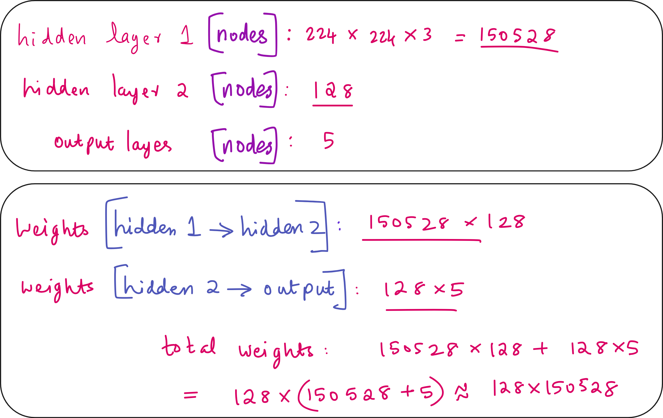
So compared to the linear model that has 750k trainable parameters, the neural network has 19 million trainable parameters.

So our hope is that these parameters can capture the patterns in the image data that helps us improve classification accuracy.

NOTE: Here we are ignoring bias because the number of bias parameters are anyway a small fraction of the number of weights. But if you want a highly accurate estimate of trainable parameters, you should also use bias.

2 hidden layer NN architecture

The below figure shows the input and output data dimensions for each layers.

We our current 2 hidden layer architecture, we can mathematically express our neural network as shown below.

But here, adding the 2nd hidden layer did not accomplish anything special because we can expand the above expression and condense the neural network to effectively just one layer.

Introduce activation function

If the introduction of second layer has to be any useful, we should add activation function. Only then the model can learn the non-linear patterns in the dataset.

It is fairy easy to introduce activation function to any layer in Keras as shown below.

There are many popular activation functions like sigmoid, ReLU, tanh etc.

In our model, we introduce ReLU because the gradient of ReLU is constant for all positive values of ReLU. This (hopefully) helps is better model training because weights will get modified faster.

Steps involved in building the model

In this series of steps, everything remains the same as the linear model except the presence of the 2nd hidden layer and the ReLU activation function after the 2nd hidden layer.

Here is the code for the steps till image visualization

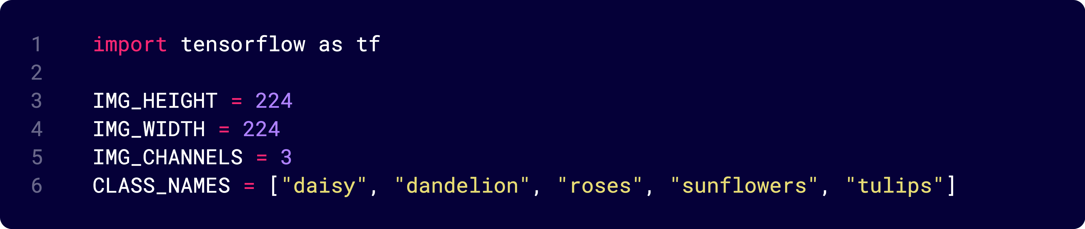
import tensorflow as tf

IMG_HEIGHT = 224
IMG_WIDTH = 224
IMG_CHANNELS = 3
CLASS_NAMES = ["daisy", "dandelion", "roses", "sunflowers", "tulips"]

def read_and_decode(filename, resize_dims):
    # 1. Read the raw file
    img_bytes = tf.io.read_file(filename)
    # 2. Decode image data
    img = tf.image.decode_jpeg(img_bytes, channels=IMG_CHANNELS)
    # 3. Convert pixel values to floats in [0, 1]
    img = tf.image.convert_image_dtype(img, tf.float32)
    # 4. Resize the image to match desired dimensions
    img = tf.image.resize(img, resize_dims)
    return img

def parse_csvline(csv_line):
    # record_defaults specify the data types for each column
    record_default = ["", ""]
    filename, label_string = tf.io.decode_csv(csv_line, record_default)

    # Load the image
    img = read_and_decode(filename, [IMG_HEIGHT, IMG_WIDTH])

    # Convert label string to integer based on the CLASS_NAMES index
    label = tf.argmax(tf.math.equal(CLASS_NAMES, label_string))
    return img, label

# Define datasets
train_dataset = (
    tf.data.TextLineDataset("gs://cloud-ml-data/img/flower_photos/train_set.csv")
    .map(parse_csvline, num_parallel_calls=tf.data.AUTOTUNE)
    .batch(16)
    .prefetch(tf.data.AUTOTUNE)
)

eval_dataset = (
    tf.data.TextLineDataset("gs://cloud-ml-data/img/flower_photos/eval_set.csv")
    .map(parse_csvline, num_parallel_calls=tf.data.AUTOTUNE)
    .batch(16)
    .prefetch(tf.data.AUTOTUNE)
)

for image_batch, label_batch in train_dataset.take(1):
    print("Image batch shape:", image_batch.shape)
    print("Label batch shape:", label_batch.shape)
    print("Labels:", label_batch.numpy())

import matplotlib.pyplot as plt

for image_batch, label_batch in train_dataset.take(2):
    # Take the first image from the batch
    first_image = image_batch[0]
    first_label = label_batch[0]

    # Convert tensor to numpy array
    plt.imshow(first_image.numpy())
    plt.title(f"Label: {CLASS_NAMES[first_label]}")
    plt.axis('off')
    plt.show()

Neural network training

Now let us define the neural network architecture once again, perform the training and validation.

New model with 2 hidden layers + activation function

from tensorflow import keras
from tensorflow.keras.optimizers import Adam

model = tf.keras.Sequential([
tf.keras.layers.Flatten(input_shape=(IMG_HEIGHT, IMG_WIDTH, 3)),
tf.keras.layers.Dense(128, activation = 'relu'),
tf.keras.layers.Dense(len(CLASS_NAMES), activation='softmax')
])

Training and validation

EPOCHS = 5

history = model.fit(
    train_dataset,
    validation_data=eval_dataset,
    epochs=EPOCHS
)

Plotting accuracy and loss

import matplotlib.pyplot as plt

plt.plot(history.history["loss"], label="Training Loss")
plt.plot(history.history["val_loss"], label="Validation Loss")
plt.xlabel("Epoch")
plt.ylabel("Loss")
plt.legend()
plt.show()

plt.plot(history.history["accuracy"], label="Training Accuracy")
plt.plot(history.history["val_accuracy"], label="Validation Accuracy")
plt.xlabel("Epoch")
plt.ylabel("Accuracy")
plt.legend()
plt.show()

Results: Our expectation vs/ reality

We might expect that adding layers will improve the model and thus lower the loss.

That is, indeed, the case. The cross-entropy loss for the linear model is on the order of 10, it is on the order of 2 for the neural network.

However, the accuracies are pretty similar, indicating that much of the improvement is obtained by the model driving probabilities like 0.7 to be closer to 1.0 than by getting items misclassified by the linear model correct.

How come the loss decreased by an order of magnitude, but the accuracy did not change much?

This is a great question to ask yourself.

Firstly let us consider the cross entropy loss function.

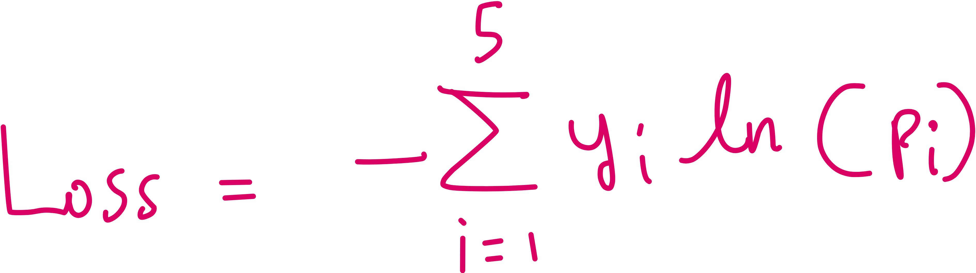
Here, i runs from 1 to 5 because there are 5 classes.

CLASS_NAMES = ["daisy", "dandelion", "roses", "sunflowers", "tulips"]

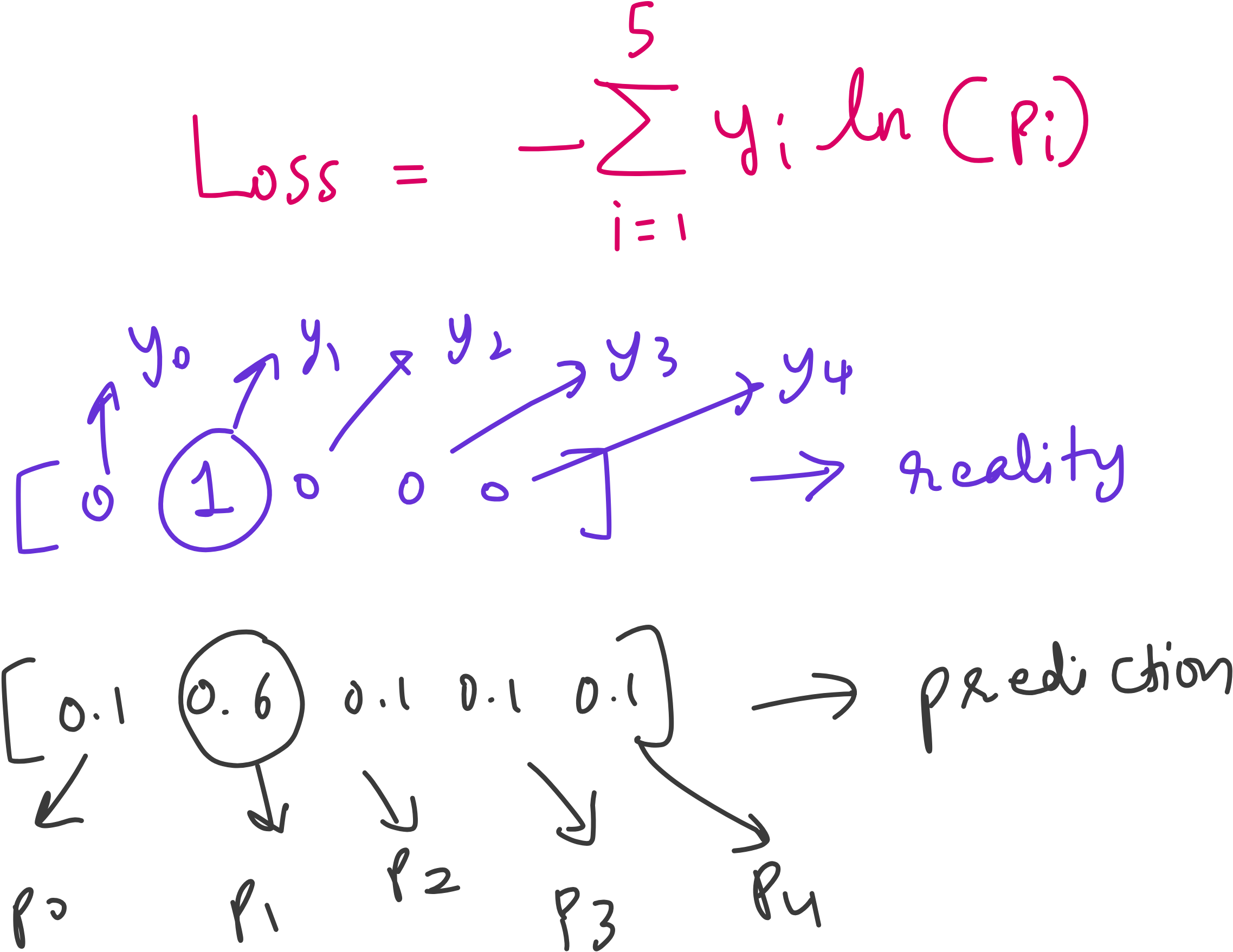
Say out label vector is y = [0 0 1 0 0]

This means the particular image whose label is the above vector is a dendelion.

Now what can a prediction by the neural network look like?

Say the prediction looks like p = [0.1 0.6 0.1 0.1 0.1]

This will result in a Loss = -1*log2(0.6) = 0.73.

The loss is 0.73, but the prediction is still correct. Because in the prediction, the index corresponding to dandelion has the highest value.

Now what if the prediction was p = [0.025 0.90 0.025 0.0.025 0.025]?

Then Loss = -1*log2(0.90) = 0.15. Loss decreased, but the predicted class remains the same - dandelion.

What if the predicted p = [0.0125 0.95 0.0125 0.0.0125 0.0125]?

Then Loss = -1*log2(0.90) = 0.075.

So when you compare p = [0.1 0.6 0.1 0.1 0.1] v/s p = [0.0125 0.95 0.0125 0.0.0125 0.0125] the Loss decrease by an order of magnitude (from 0.73 to 0.075), but the predicted class remains the same - dandelions.

This is exactly what happened in our neural network. The neural network is now able to predict the correct classes with higher confidence, but the number of correct classifications have not increased.

This is why even though the loss has decreased by an order of magnitude, the accuracy has not changed much.

So adding an extra layer did not work. What else can we do?

Parmeters v/s hyperparameters

Parameters

• Learned from data during training

• Define the model's internal state

• Examples:

  • Weights and biases in a neural network

  • Coefficients in linear regression

• Updated by optimization algorithms (like gradient descent)

Think of parameters as what the model learns.

Hyperparameters

• Set before training begins

• Control the training process or model structure

• Examples:

  • Learning rate

  • Number of layers or neurons

  • Batch size

  • Epochs

  • Activation functions

  • Optimizer type

Think of hyperparameters as what you set to help the model learn well.

Learning rate

It is very easy to change the learning rate in our model. The default learning rate for Adam optimizer in Keras, unless we specify, is 0.001.

Image size

We can try resizing the image to smaller dimension to check if our accuracy is improving because now the models does not have too much to learn. But this is a double edged sword because resizing can cause significant loss in information. Thus although training may become faster, accuracy may suffer.

This is the code snippet where we can re-define the image height and width.

Batch size

In machine learning (especially in deep learning), batch size refers to the number of training examples the model sees before updating the weights once.

There are three modes of learning based on batch size:

1. Stochastic Gradient Descent (SGD):
   Batch size = 1 (weights are updated after every sample).
   Pros: Noisy but can escape local minima.
   Cons: Slow and unstable.

2. Batch Gradient Descent:
   Batch size = size of the entire training dataset.
   Pros: Stable and deterministic.
   Cons: Memory-intensive and slow to update.

3. Mini-Batch Gradient Descent (most common):
   Batch size = a small number (like 32, 64, 128, etc.)
   Pros: Good tradeoff between efficiency and stability.

What's an Optimal Batch Size?

There is no one-size-fits-all, but some general tips:

Typical choices:

• 32 or 64: Good starting points.

• 128 or 256: If your GPU has good memory.

• 512 or 1024+: For large datasets and powerful GPUs (like in foundation models).

Things to consider:

• Memory limitations: Larger batches consume more GPU RAM.

• Generalization: Smaller batch sizes often generalize better.

• Training speed: Larger batches = fewer updates per epoch, which may train faster.

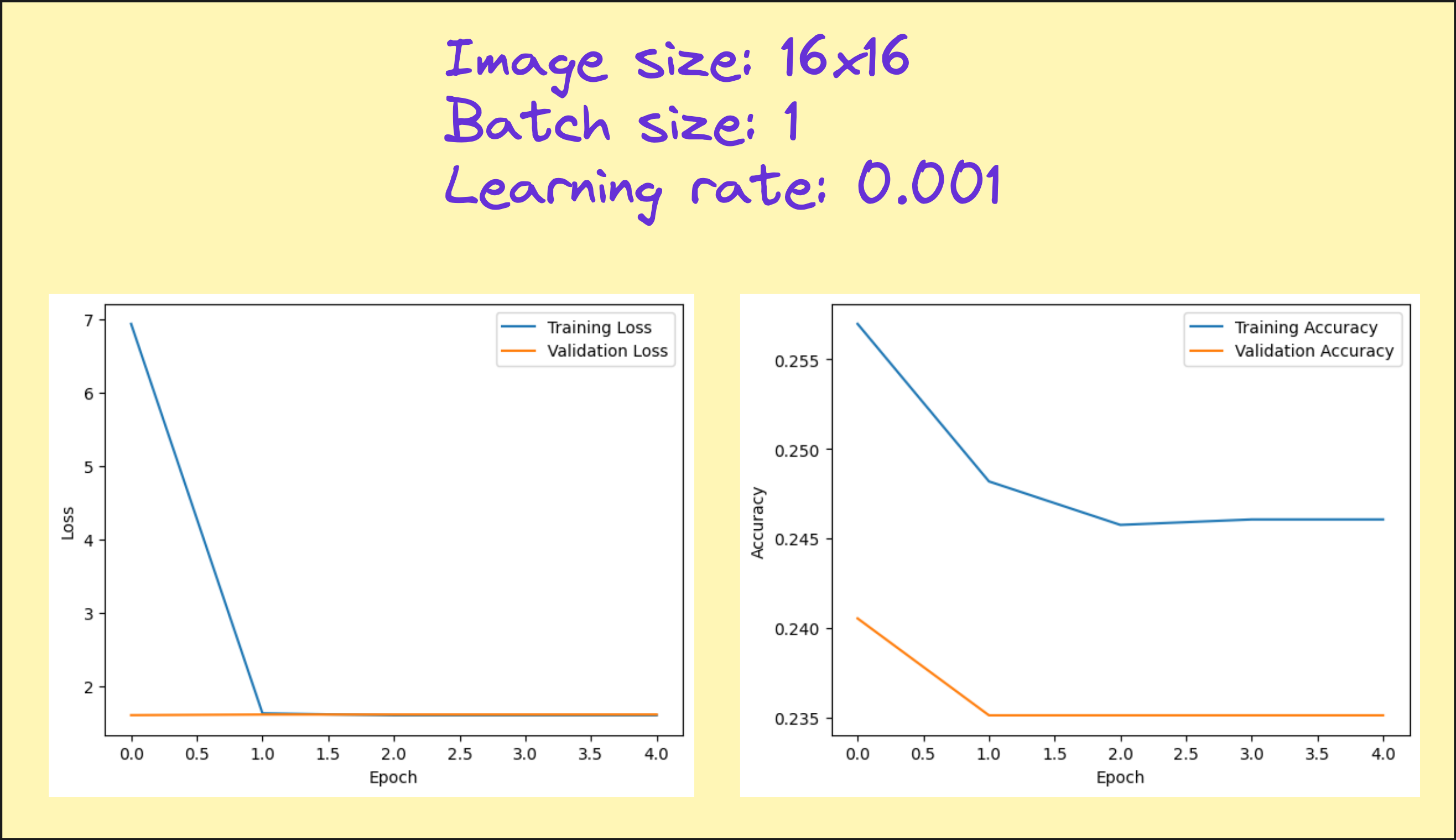
Results from our hyperparameter tuning (only image size and batch size)

Look at the loss and accuracy plots from various experiments I performed. You can see that there is no significant improvement in accuracy, but in several cases, we have managed to cut down the loss significantly, indicating more confident predictions. So although our metric if interest (accuracy) is not improving, this neural network model is doing something better than the linear model.

Still not that better. What else can be done?

So what else can be done to make our neural network better? We are yet to do the following.

• Change the learning rate

• Regularization [to reduce overfitting]

• Dropout [to reduce overfitting]

• Deeper neural network [to learn more features in the image]

We will explore this in the next article on this topic.

Lecture video

I have made a lecture video on this topic and hosted it on Vizuara’s YouTube channel. Do check this out. I hope you enjoy watching this lecture as much as I enjoyed making it.

Here is the link to the Colab notebook: https://colab.research.google.com/drive/1m4JuGfPdqL59SF1X_6lcRT-NEKy4azov?usp=sharing

If you are interested in AI/ML foundations, check out these resources

1. Foundational courses: https://vizuara.ai/self-paced-courses

2. SciML research bootcamp: https://flyvidesh.online/ml-bootcamp/

3. GenAI professional bootcamp: https://flyvidesh.online/gen-ai-professional-bootcamp