From One-Hot encoding to meaning

Build Word2Vec from scratch and understand every layer

“You shall know a word by the company it keeps.” — J.R. Firth

This idea powers one of the most influential breakthroughs in Natural Language Processing: Word2Vec. In this article, not only will you understand the theory and math behind Word2Vec's architecture, but you will also learn how to implement it entirely from scratch.

If you are an AI researcher, NLP enthusiast, or an aspiring ML engineer, this deep dive will empower you to build your own custom word embeddings and understand their structure, training, and utility.

Prerequisites

Before diving in, make sure you are familiar with:

• One-Hot Encoding

• Neural Networks (basics of layers, weights, activations)

• Cross-Entropy Loss

• Matrix multiplication

If not, no worries, this article will gently reinforce those concepts where needed.

---

The Evolution: From symbolic to distributed representations

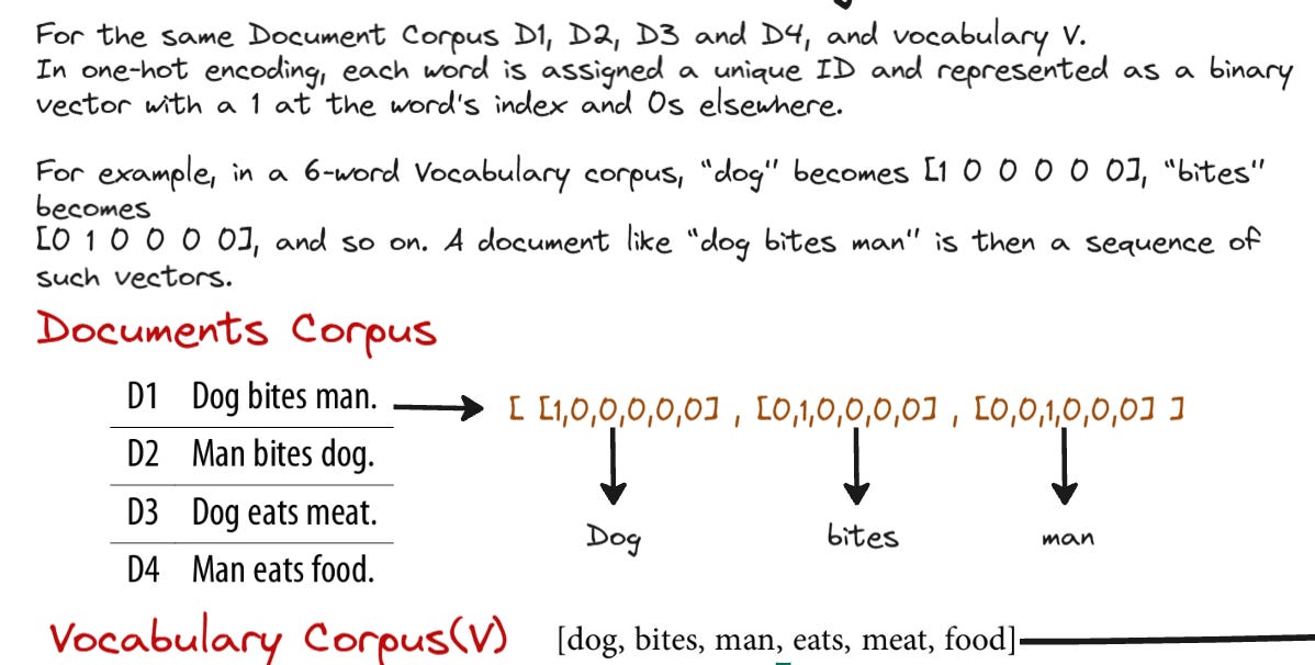
NLP began with symbolic representations like One-Hot Encoding, Bag-of-Words, and TF-IDF. But these techniques treat words as isolated symbols, with no understanding of context.

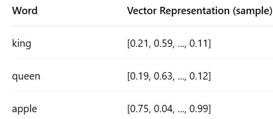
Enter distributed representations, where words are represented as dense vectors in continuous space, capturing both semantic and syntactic similarities.

Distributed Representations

---

What is Word2Vec?

Word2Vec is a shallow, two-layer neural network architecture that learns word embeddings using context.

There are two main architectures:

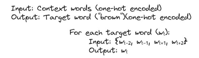
• CBOW (Continuous Bag of Words) – predicts a target word from context

• Skip-Gram – predicts context from a target word

We will focus on CBOW, and more importantly, build it from scratch.

CBOW: Mathematical formulation

Let us break this into layers and their respective mathematical operations.

Raw Text Corpus -> "The quick brown fox jumps over the lazy dog"

Data Preparation from the raw text corpus

After the preprocessing of the raw text corpus, we split it into correct structure to feed into the Model as input.

1. Input Layer : One-Hot Encoding

Let V be the vocabulary size. Each word w is represented as a one-hot vector":

2. Embedding Layer – Matrix Lookup

Let the embedding matrix be:

Where:

• V: Vocabulary size

• D: Embedding dimension (e.g., 100 or 300)

For each context word xi, its embedding is:

The embeddings of each of the context words are used as the input for aggregation

If we use C context words, we aggregate their embeddings:

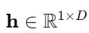
h is our hidden vector, representing the context.

3. Output Layer – Softmax Prediction

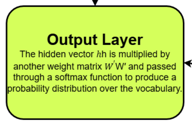
Now we transform h into a vocabulary-sized prediction vector:

Let the output weight matrix be: (Here W’ is represented as U)

Then,

Apply softmax to get the probability of each word:

Here, the softmax layer will give us the output of the one-hot encoded representations of the predicted word.

4. Loss function – Cross entropy

Let y be the one-hot vector for the true target word. Then the loss is:

Since y is one-hot, this simplifies to:

This metric says how close are the predictions to the actual word positions in the one-hot encoded representations. As here, the ground truth will be presented in one-hot encoded format and the prediction will be in one-hot encoded format as an output from softmax layer.

5. Training – backpropagation & weight update

We update the weights using stochastic gradient descent:

Where η (eeta/ita) is the learning rate.

Both the input layer’s weight matrix and the output layer’s weight matrix values are updated during back propagation to minimize the cross entropy loss and ultimately get the perfect embedding vector representations of the words.

In general, this output layer is essentially used as a decoder to verify whether the “h” context vector is representing the corresponding word or not.

Overall Architecture

Implementation summary (pytorch)

We:

• Use WikiText-2 corpus

• Tokenize and build vocab (min frequency = 5)

• Construct custom CBOWDataset with context window = 2

• Use nn.Embedding and nn.Linear

• Train on GPU using Adam and CrossEntropyLoss

• Extract learned embeddings post training

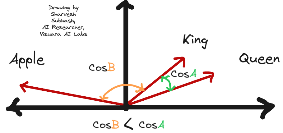
  Cosine similarity: Do the vectors make sense?

  After training, we compare words like:

  

  Even on partially trained models, we observe this:

  

  

  When we project the embedding values of the words “King” and “Queen”, the projections appear closer to each other due to their contextual similarity that the projections between “King” and “Apple”.

  Cosine of acute angle → Positive ratio, Cosine of obtuse → Negative ratio.

  So, the Cosine similarity of the two word ( King and Queen)vectors is the proof that Word2Vec embeddings capture semantic similarity inherently through training!

  🤯 Why this matters

  By building Word2Vec yourself, you will understand:

• How text transforms into meaning.

• How embeddings are mathematically grounded.

• Why Word2Vec was a turning point in NLP.

  🎥 Prefer visual learning?

  I have explained every concept and equation above with visuals and implemented the full Word2Vec CBOW model from scratch in PyTorch on our Vizuara YouTube channel.

  Watch the full lecture here →
  👉

  Includes:

  • Complete Colab notebook

  • Hands-on training demo

  • Cosine similarity checks

  • Custom similarity functions

  • Real vector extraction

Final challenge for you

Try modifying the model:

• Switch from CBOW to Skip-Gram

• Use Negative Sampling instead of Softmax

• Train on your own text corpus (like Reddit or Twitter)

  👉 Don’t just use Word2Vec. Build it. Understand it. Own it.