
A shallow neural network is better than a monkey
A simple neural network with 1 hidden layer, no activation function and no convolution


Neural networks have revolutionized how machines understand and classify images, but what happens when we strip them down to their simplest form?
In this article, we will build a shallow neural network for image classification - without any activation functions.
This hands-on exercise will reveal fascinating insights into how neural networks learn, why activation functions matter, and how the depth of a network affects classification accuracy. By the end, you will also see why convolutional operations are essential for image recognition. .
Before doing anything else, let us first make sure we have the dataset prepared.
Our dataset
Consider the famous 5-flowers dataset containing real-world images of the following flower categories:
Daisies
Dandelions
Roses
Sunflowers
Tulips

Each photograph is a standard JPEG image - just like the ones you take on your smartphone - stored in different folders by flower type. Each flower category has 1000 images.
The dataset and images, created by Google, are available in the public GitHub repo hosted at this link: https://github.com/GoogleCloudPlatform/practical-ml-vision-book and also in the famous O’Reilly book Practical Machine Learning for Computer Vision.

Let us read the dataset
Since our 5-flower dataset are just everyday JPEG images, we need to convert them into a format that is easy for ML models in Python to process. The reading process involves the following steps:
Load the file: Grab the JPEG file from a disk or a remote location (eg:- Kaggle: https://www.kaggle.com/datasets/kausthubkannan/5-flower-types-classification-dataset)
Decode: Turn the compressed JPEG files into the pixel values (RGB).
Scale: Convert pixel values to a floating-point range between 0 and 1. Initially, the range of pixel values for R, G, and B channels will be 0-255.
Resize: Make sure all images are of the same dimension, say 224×224, so the model can handle them uniformly. This is a very important step in data preprocessing.
It is also crucial to verify that you are reading the images correctly. You can’t check all images, but you can visual check a few images to confirm they aren’t rotated or flipped accidentally! Visualizing images is a good sanity check in any computer vision project.
In this article, we will be using TensorFlow, NumPy and Matplotlib libraries from Python. But going ahead further, it is very import to understand what exactly do these 3 libraries do?

What are TensorFlow, NumPy and Matplotlib?
1. TensorFlow
TensorFlow is an open-source deep learning framework developed by Google. It is widely used for Machine Learning (ML) and Deep Learning (DL) applications, including neural networks.
Key features
Efficiently handles large-scale numerical computations.
Supports CPU and GPU acceleration.
Used for training and deploying ML models.
2. NumPy
NumPy (Numerical Python) is a library for numerical computing in Python. It provides support for multi-dimensional arrays, linear algebra, and mathematical operations.
Key features
Efficient array operations using ndarray.
Vectorized computations (faster than traditional Python lists).
Commonly used for data preprocessing in ML.
3. Matplotlib
Matplotlib is a data visualization library used for creating graphs, plots, and charts.
Key features
Supports line plots, bar charts, histograms, scatter plots, etc.
Works well with NumPy and Pandas.
Useful for visualizing data in ML and AI.
Now let us read the image data.
A key difference between NumPy & TensorFlow
In Python, NumPy is the standard library for numerical computations, providing support for n-dimensional arrays. However, NumPy operations are not hardware-accelerated by default, which can be a limitation for large-scale computations.
For example, a 1D NumPy array with a shape of (4) can be created as follows:
import numpy as np

x = np.array([2.0, 3.0, 1.0, 0.0])
Similarly, a 5D array of zeros (with five dimensions in its shape) can be created using:
import tensorflow as tf

tx = tf.convert_to_tensor(x, dtype=tf.float32)
Conversely, you can convert a TensorFlow tensor back into a NumPy array:
x = tx.numpy()While NumPy arrays and TensorFlow tensors are mathematically equivalent, they differ in execution:
NumPy computations run on the CPU.
TensorFlow operations utilize a GPU (if available), making them significantly faster for large-scale computations.
For instance, performing element-wise multiplication:
x = x * 2.1  # Runs on CPU
tx = tx * 2.1  # Runs on GPU (if available), making it more efficient
To maximize computational efficiency:
Use TensorFlow operations instead of NumPy whenever possible.
Vectorize computations, especially when processing large datasets (e.g., images), to perform batch operations rather than numerous small scalar calculations.
Steps involved in reading image data
Step 1: Load the CSV file, read the images, and create a TensorFlow dataset
You can run the below code in Google Colab.
import tensorflow as tf

IMG_HEIGHT = 224
IMG_WIDTH = 224
IMG_CHANNELS = 3
CLASS_NAMES = ["daisy", "dandelion", "roses", "sunflowers", "tulips"]

def read_and_decode(filename, resize_dims):
    # 1. Read the raw file
    img_bytes = tf.io.read_file(filename)
    # 2. Decode image data
    img = tf.image.decode_jpeg(img_bytes, channels=IMG_CHANNELS)
    # 3. Convert pixel values to floats in [0, 1]
    img = tf.image.convert_image_dtype(img, tf.float32)
    # 4. Resize the image to match desired dimensions
    img = tf.image.resize(img, resize_dims)
    return img

def parse_csvline(csv_line):
    # record_defaults specify the data types for each column
    record_default = ["", ""]
    filename, label_string = tf.io.decode_csv(csv_line, record_default)

    # Load the image
    img = read_and_decode(filename, [IMG_HEIGHT, IMG_WIDTH])

    # Convert label string to integer based on the CLASS_NAMES index
    label = tf.argmax(tf.math.equal(CLASS_NAMES, label_string))
    return img, label
The below code will create testing and validation dataset by passing the train_set.csv and eval_set.csv to the parse_csvline() function.
# Define datasets
train_dataset = (
    tf.data.TextLineDataset("gs://cloud-ml-data/img/flower_photos/train_set.csv")
    .map(parse_csvline, num_parallel_calls=tf.data.AUTOTUNE)
    .batch(16)
    .prefetch(tf.data.AUTOTUNE)
)

eval_dataset = (
    tf.data.TextLineDataset("gs://cloud-ml-data/img/flower_photos/eval_set.csv")
    .map(parse_csvline, num_parallel_calls=tf.data.AUTOTUNE)
    .batch(16)
    .prefetch(tf.data.AUTOTUNE)
)
What is happening here?
We read each row of the CSV file, which contains a file path and the flower label (label meaning which flower category does the image belong to).
parse_csvlinecallsread_and_decodeon the JPEG file.We batch the data so the model can process multiple images in one go.
When you create a tf.data.Dataset pipeline like this, it does not automatically print or return anything to the console. The code itself only defines the dataset and how to read and batch the data. It does not consume the dataset yet, which is why it may appear that there is “no output.”
To confirm that your pipeline is working correctly, you can do one of the following:
Step 2: Create a batch dataset of images
The below code will fetch the first batch of dataset that contains 16 images.
for image_batch, label_batch in train_dataset.take(1):
    print("Image batch shape:", image_batch.shape)
    print("Label batch shape:", label_batch.shape)
    print("Labels:", label_batch.numpy())
Step 3: Visualize a single image example
The below code uses Matplotlib to visualize the picture of a sample datapoint. Here the picture is that of a “daisy” flower.
import matplotlib.pyplot as plt

for image_batch, label_batch in train_dataset.take(2):
    # Take the first image from the batch
    first_image = image_batch[0]
    first_label = label_batch[0]

    # Convert tensor to numpy array
    plt.imshow(first_image.numpy())
    plt.title(f"Label: {CLASS_NAMES[first_label]}")
    plt.axis('off')
    plt.show()
Great! Our TensorFlow pipeline for reading the images is working.
Step 4: Visualize a batch of images
import matplotlib.pyplot as plt

# Take one batch from the dataset
for image_batch, label_batch in train_dataset.take(2):
    fig, axes = plt.subplots(4, 4, figsize=(10, 10))  # Create a 4x4 grid

    for i in range(16):  # Loop over the first 16 images
        ax = axes[i // 4, i % 4]  # Determine grid position
        ax.imshow(image_batch[i].numpy())  # Convert tensor to numpy array
        ax.set_title(f"Label: {CLASS_NAMES[label_batch[i]]}")
        ax.axis("off")  # Hide axes

    plt.tight_layout()
    plt.show()
Now that we know our TensorFlow dataset pipeline is ready, we can build our first ML model to classify flower images.
Linear neural network for image classification — [no activation, no convolution]
The 5-flowers dataset gives us something concrete to experiment with. And while we might know that simple linear models aren’t best suited for images, it is a great introduction to how ML generally works.
Why are we calling our first model “linear”? Because we will not be using any activation functions.
Flattening the image
In a linear model, every pixel is treated as an individual input. So, if your image is 224×224 pixels with three color channels (R, G, B), you end up with 224×224×3 total inputs - each pixel is a separate number. You flatten these into a single long vector because a linear model doesn’t “see” any adjacency or shape - just raw intensity values.
The dense (fully-connected) layer
All those input pixels (224x224x3 per image) feed into a “dense” layer. This layer outputs a separate score (or logit) for each flower category. The model looks like this.

Behind the scenes, the Dense layer calculates Y = softmax(B + W * X), where:
X is your flattened image data,
W is the trainable weight matrix,
B is a bias term,
Y is the output vector of 5 scores, one for each flower type.
NOTE: It might seem contradictory at first that the model does use softmax, which is technically an activation function. However, the reason we say "no activation function" in this context is because we are not applying any non-linearity before the final output layer.
The Dense layer in this model is purely linear. It just applies a matrix multiplication (W * X) and adds a bias (B). Normally, deep learning models introduce non-linearity using activation functions like ReLU, tanh, or sigmoid in hidden layers, which allow the model to learn more complex patterns. Here, no activation function is applied between layers, so the entire transformation is linear.
Defining a linear model using Keras
A linear model treats each pixel value as a separate input. We flatten the images to a single dimension, then connect it directly to five output scores (one for each flower type).
This following Keras code implements the linear model with a flatten :
from tensorflow import keras

model = keras.Sequential([
    keras.layers.Flatten(input_shape=(IMG_HEIGHT, IMG_WIDTH, IMG_CHANNELS)),
    keras.layers.Dense(len(CLASS_NAMES), activation="softmax")
])

model.compile(
    optimizer="adam",
    loss=keras.losses.SparseCategoricalCrossentropy(from_logits=False),
    metrics=["accuracy"]
)
Flatten layer: Reshapes each image of shape [224, 224, 3] to a 1D vector of size 224 × 224 × 3.
Dense layer: Outputs five scores, one per flower category. The softmax activation converts these scores to probabilities that sum to 1.
By the way, what is Keras?
Keras is an open-source deep learning framework that provides an easy-to-use, high-level API for building and training neural networks. It is written in Python and runs on top of deep learning backends like TensorFlow.

While TensorFlow is a powerful deep learning framework, Keras provides a simpler, more intuitive interface for building and training models. In short, Keras helps you use TensorFlow in an easier way.
Training the linear model
To train your model, you need:
An optimizer (like Adam) that adjusts weights based on the gradient of the loss.
A loss function (for classification, cross-entropy is typically used).
An evaluation metric (like accuracy) to measure how many predictions match the true label.
As you train:
You repeatedly pass batches of images through the model.
Compare predictions to the correct flower labels.
Calculate how “off” the predictions are via the loss function.
Update the model parameters in the direction that reduces that loss.
We can now train this model and see how it performs on our training and evaluation splits:
EPOCHS = 10

history = model.fit(
    train_dataset,
    validation_data=eval_dataset,
    epochs=EPOCHS
)train_datasetprovides the images and labels during training.validation_datais used for calculating metrics on unseen data to monitor overfitting.The training loop will run for 10 epochs.
Now that the training is done, let us visualize the training and validation losses as a function of epochs.
Visualizing the training and validation losses
import matplotlib.pyplot as plt

plt.plot(history.history["loss"], label="Training Loss")
plt.plot(history.history["val_loss"], label="Validation Loss")
plt.xlabel("Epoch")
plt.ylabel("Loss")
plt.legend()
plt.show()

plt.plot(history.history["accuracy"], label="Training Accuracy")
plt.plot(history.history["val_accuracy"], label="Validation Accuracy")
plt.xlabel("Epoch")
plt.ylabel("Accuracy")
plt.legend()
plt.show()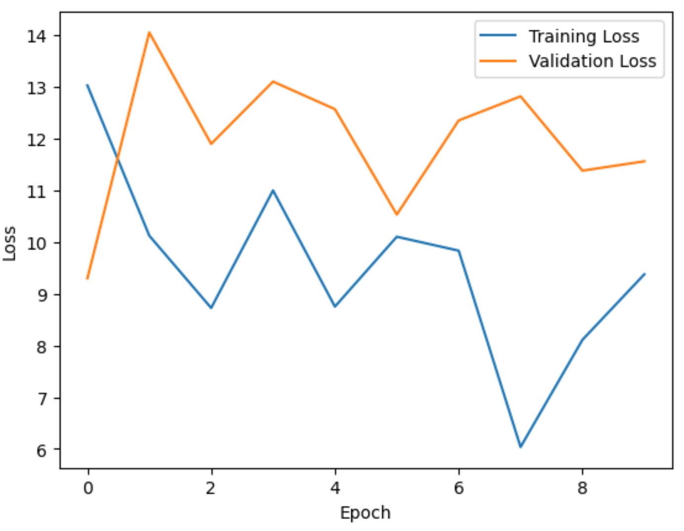

Outcome
A linear model usually yields a modest accuracy on image tasks because it has no concept of shape or spatial relationships. The accuracy isn’t spectacular - somewhere around 40-45%. But that is enough to show the training workflow in action. Please note that the worst accuracy possible in a 5-class classification is 0.2 - equivalent to the accuracy of random guessing.
Making predictions on some sample validation data
Let us now try to make some predictions on sample validation data. Validation data was not exposed to the neural network while training.
import numpy as np
import matplotlib.pyplot as plt
import math

# Take exactly one batch from the evaluation dataset
for images, labels in eval_dataset.take(1):
    # Get model predictions for this batch
    batch_predictions = model.predict(images)
    predicted_indices = np.argmax(batch_predictions, axis=1)

    # Number of images in this batch
    num_images = images.shape[0]

    # Configure how many images to display per row
    num_cols = 4
    num_rows = math.ceil(num_images / num_cols)

    # Create a figure with a suitable size
    plt.figure(figsize=(12, 3 * num_rows))

    for i in range(num_images):
        plt.subplot(num_rows, num_cols, i + 1)

        # Display the image
        plt.imshow(images[i].numpy())
        plt.axis('off')

        # Get predicted and actual class names
        pred_class = CLASS_NAMES[predicted_indices[i]]
        actual_class = CLASS_NAMES[labels[i].numpy()]

        # Show both predicted and actual labels as title
        plt.title(f"Pred: {pred_class}\nActual: {actual_class}", fontsize=10)

    # Adjust spacing to avoid overlapping titles, etc.
    plt.tight_layout()
    plt.show()
Observations and limitations
A purely linear model, as expected, will not capture intricate patterns in the images. You will often see validation accuracy stall around 40 to 50 percent, which is above random chance (20% for five classes) but not very high. This illustrates that a simple flatten-and-dense approach lacks the spatial awareness of more sophisticated methods like convolutional neural networks.
In the next article, we will build a deep neural network and see how well it can perform compared to this shallow neural network.
Here is the Google Colab code for the entire linear neural network pipeline: https://colab.research.google.com/drive/15D91NChzSrEM2kTr9E8GI6l1FGvu6men?usp=sharing
Here is the Google Colab code for comparing the implementation speed of Tensoflow vs Numpy: https://colab.research.google.com/drive/1WaFuI2T5gUvaewAM3XiLiIrogaRLjROV?usp=sharing
Lecture video
I have released a lecture video on this topic on Vizuara’s YouTube channel. Do check this out. I hope you enjoy watching this lecture as much as I enjoyed making it.
3 things we can do to improve our model
1) Introduce “deep” neural network instead of “shallow” neural network
In a shallow neural network you have an input layer, one or two hidden layers, and an output layer.
In a deep neural network you have an input layer, many hidden layers (sometimes dozens or even hundreds), and an output layer. Each layer can learn increasingly abstract features from raw input.

2) Use non-linear activation function
An activation function is a mathematical function used in neural networks to introduce non-linearity, allowing the network to learn complex patterns in the data. It determines whether a neuron should be activated based on its input.

Introduce non-linearity: Without an activation function, a neural network would behave like a simple linear regression model, limiting its ability to solve complex problems.
Enable Deep Learning: Deep networks rely on activation functions to capture intricate relationships in data.
3) Use convolutional neural network for learning intricate patterns from the images
The below image is an example of convolution operation using a 3x3 filter applied on a 5x5 matrix.

This process is called convolution (more precisely, cross-correlation if we don’t rotate the kernel, but in most computer-vision libraries, we call it convolution for simplicity).
For each pixel, you:
Overlay the filter on the local neighborhood of that pixel (commonly a 3×3 or 5×5 region).
Multiply each filter entry by the corresponding pixel intensity.
Sum all these products to produce a single new intensity (or gradient value, or some other measure).