A simple Machine Learning model for forecasting the pandemic

Epidemiology + Machine Learning

This article is about Scientific Machine Learning - an emerging field that combines the interpretability of mechanistic models with the predictive power of ML models.

Let us learn using a simple example of COVID virus spreading. How would we model the spread of COVID in a population?

The "science" of virus spread - SIR model

Let us see how scientific machine learning can be used to predict the spread of infectious diseases like COVID-19 by combining epidemiological models with the power of machine learning.

Specifically, we focus on the SIR model, one of the simplest yet foundational models in epidemiology.

The SIR model categorizes a population into three compartments: Susceptible (S), Infected (I), and Recovered (R).

Initially, the entire population is susceptible except for a few infected individuals. As the virus spreads, susceptible individuals become infected, and over time, infected individuals recover and gain immunity.

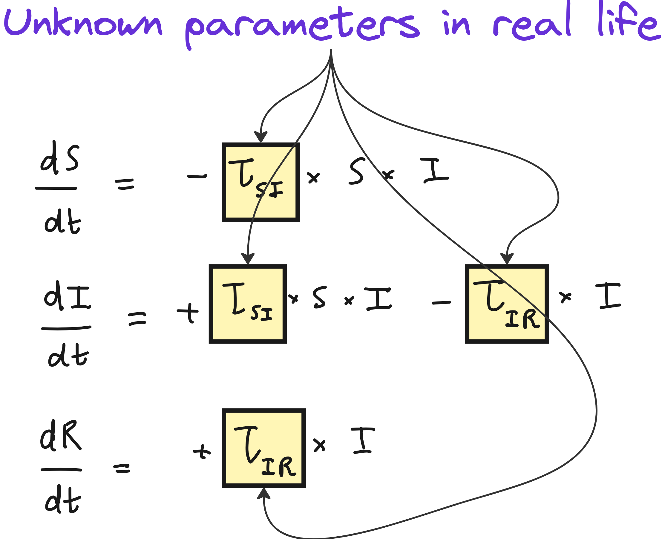
This transition is modeled using a system of three ordinary differential equations, each representing the rate of change of the S, I, and R populations. The model uses parameters like τ_SI (the rate at which susceptible people become infected) and τ_IR (the recovery rate).

The problem with SIR model

The SIR model has serious limitations. We are ignoring real life situations like hospitalizations, deaths, quarantine etc. But even if we were to ignore those factors, the biggest problem with SIR model is that the interaction parameters τ_SI (the rate at which susceptible people become infected) and τ_IR (the recovery rate) are difficult to estimate in real life.

This limitation is where machine learning proves valuable - by learning these parameters from large datasets across cities and regions, we can make better predictions about the progression of an outbreak.

Machine Learning to make predictions

We can use neural networks to create a mapping from initial conditions such as S(t=0), I(t=0) and R(t=0) to the number of infections at the end of a month. For this we will need real world data from different regions of the world.

However, traditional machine learning models are often black boxes and don’t leverage the known structure of these scientific equations.

Problem with traditional ML

In the SIR model, we have some information. Although the interaction parameters maybe unknown, we can still deduce the presence of S, I and R terms in the 3 equations using logic. So why should we throw away this knowledge and just use a black box?

Enter Scientific ML

Scientific machine learning bridges this gap by integrating known physical or epidemiological relationships (like those in the SIR model) into the learning process, resulting in models that are both interpretable and more accurate, even with partially unknown parameters. This synergy offers a promising direction for modeling complex systems where domain knowledge and data can complement each other.

In SciML, we can retain the differential equations, but replace the unknown terms by neural networks.

In scientific machine learning, we enhance traditional models like the SIR epidemiological framework through Universal Differential Equations (UDEs).

Unlike black-box machine learning models that ignore domain knowledge, UDEs preserve the structure of known scientific laws - such as the system of ordinary differential equations (ODEs) in the SIR model - while replacing unknown or hard-to-estimate terms (like the interaction parameters τ_SI and τ_IR) with trainable neural networks.

UDE for SIR model

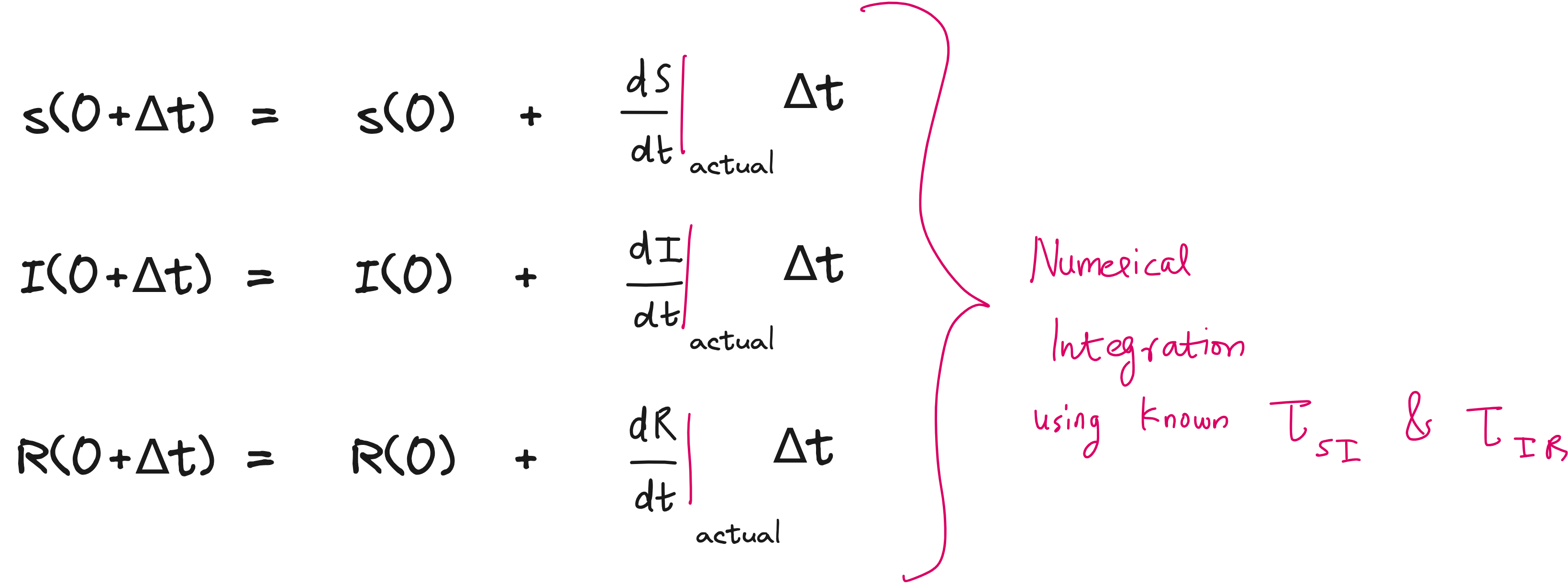
For example, instead of assuming fixed values for these parameters, UDEs use neural networks to learn and predict them based on initial inputs like the susceptible or infected population. These predicted values are then plugged into the ODEs, which are solved using numerical integration (e.g., Euler method) to compute the next state of susceptible, infected, and recovered individuals over time.

In the Universal Differential Equation (UDE) framework applied to the SIR model, two neural networks - NN1 and NN2 - are introduced to estimate the unknown interaction parameters τ_SI and τ_IR, respectively.

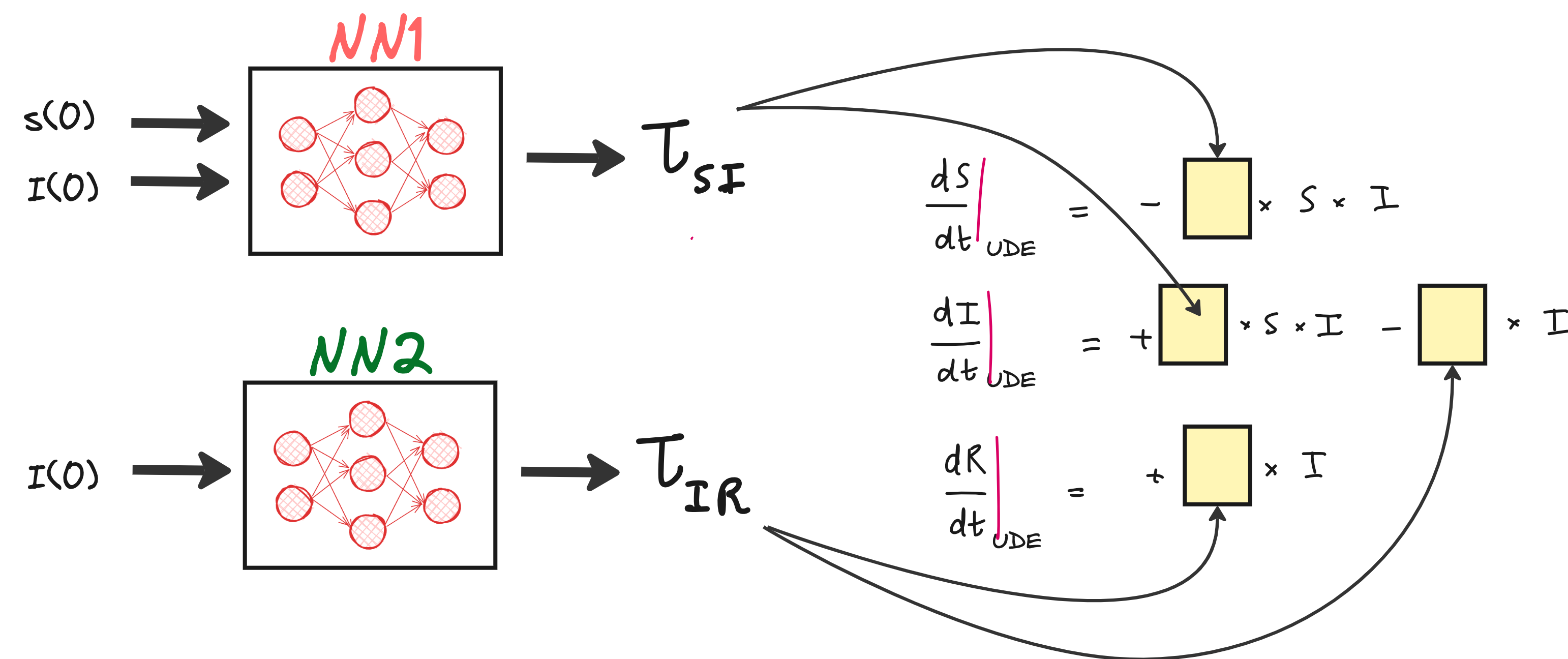
These neural networks act as functional approximators that take in certain epidemiological variables as inputs and output a scalar value representing the corresponding interaction rate at a given time.

• NN1 (Neural Network 1):

  • Inputs: The susceptible population S(t) and the infected population I(t) at a given time step.

  • Output: The estimated interaction parameter τ_SI, which governs the rate at which susceptible individuals become infected. This output is then used in the differential equations for both dS/dt and dI/dt.

• NN2 (Neural Network 2):

  • Input: The infected population I(t) at a given time step.

  • Output: The estimated interaction parameter τ_IR, which governs the rate at which infected individuals recover. This value is used in the differential equations for dI/dt and dR/dt.

These inputs are typically normalized or scaled for effective learning, and the outputs are constrained to be positive since interaction rates cannot be negative. By learning these parameters from data over time, NN1 and NN2 help the UDE dynamically adapt to different outbreak scenarios and virus behaviors, while still preserving the structure of the original SIR model.

By comparing the model's predicted trajectories with actual data-using metrics like Mean Squared Error (MSE) - the neural networks are trained via backpropagation to minimize prediction error. This hybrid approach leverages the interpretability and grounding of scientific models while capturing complex patterns through machine learning, making it ideal for forecasting real-world phenomena like virus spread where partial scientific knowledge is available but precise parameters are uncertain.

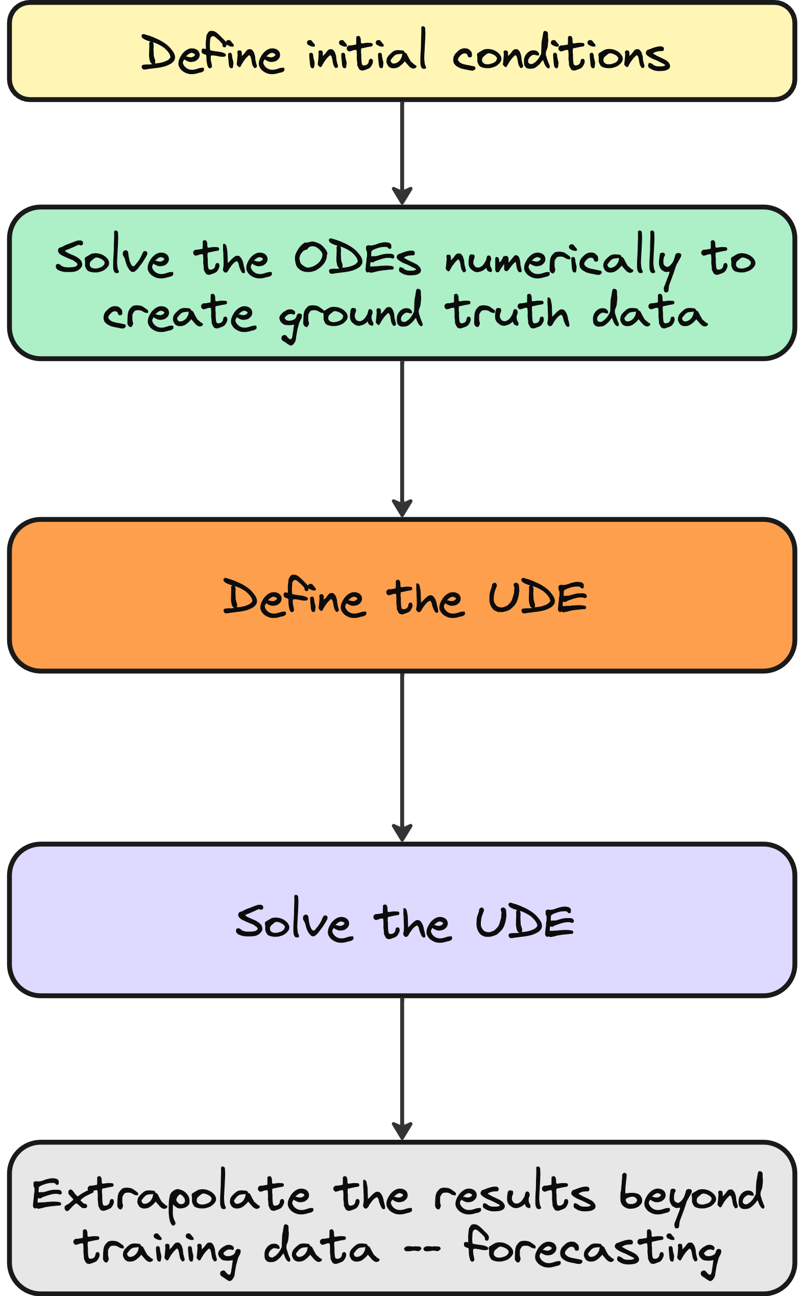
Steps involved in setting up and solving the UDE

Lecture video

I have made a lecture video on UDEs (incorporating SIR model) and hosted it on Vizuara’s YouTube channel. Do check this out. I hope you enjoy watching this lecture as much as I enjoyed making it.

If you wish to conduct research in SciML, check this out: https://flyvidesh.online/ml-bootcamp/

Code implementation in Julia

Import packages

using DifferentialEquations, Random, Lux, ComponentArrays, Optimization, OptimizationOptimJL, DiffEqFlux, Plots

Constants and initial conditions

N_days = 25  # Duration of the simulation (in days)
const S0 = 1.0  # Total population (normalized to 1.0)
u0 = [S0 * 0.99, S0 * 0.01, 0.0]  # Initial conditions: [Susceptible, Infected, Recovered]

# True infection and recovery rates (used for synthetic data generation)
p0 = [0.85, 0.1]  # [τSI (infection rate), τIR (recovery rate)]

tspan = (0.0, Float64(N_days))  # Time range for simulation
t = range(tspan[1], tspan[2], length=N_days)  # Time points for evaluation

Solving the SIR ODE for ground truth

# Define the classic SIR model as an ODE
function SIR!(du, u, p, t)
    (S, I, R) = u
    (τSI, τIR) = abs.(p)  # Ensure parameters are non-negative

    du[1] = -τSI*S*I  # dS/dt = ?
    du[2] = τSI*S*I - τIR*I  # dI/dt = ?
    du[3] = τIR*I  # dR/dt = ?
end

# Solve the ODE to generate synthetic data
prob = ODEProblem(SIR!, u0, tspan, p0)
true_sol = Array(solve(prob, Tsit5(), saveat=t))  # Solve using appropriate solver

Construct the UDE

# ============================
# 2. Constructing the UDE Model (Neural Network-driven SIR Model)
# ============================
rng = Random.default_rng()  # Random number generator for reproducibility

# Define two neural networks to learn infection and recovery rates
NN_SI = Lux.Chain(Lux.Dense(2, 10, relu), Lux.Dense(10, 1))  # Neural network for τSI
NN_IR = Lux.Chain(Lux.Dense(1, 10, relu), Lux.Dense(10, 1))  # Neural network for τIR

# Initialize neural network parameters
p1, st1 = Lux.setup(rng, NN_SI)
p2, st2 = Lux.setup(rng, NN_IR)

# Store all NN parameters in a structured format
p0_vec = (layer_1 = p1, layer_2 = p2)
p0_vec = ComponentArray(p0_vec)  # Convert to ComponentArray for optimization

# Define a softplus activation function to ensure non-negative outputs
function softplus(x)
    return log(1 + exp(x))
end

# Define the SIR Universal Differential Equation (UDE) model
function SIR_UDE!(du, u, p, t)
    (S, I, R) = u  # Extract S, I, R

    # Compute dynamic parameters using neural networks
    NNSI, _ = NN_SI([S, I], p.layer_1, st1)  # Predict τSI using NN_SI
    NNIR, _ = NN_IR([I], p.layer_2, st2)  # Predict τIR using NN_IR

    # Convert outputs to positive and stable values
    τSI = clamp(softplus(NNSI[1]), 10e-5, 1)  # Clamp τSI between min and max
    τIR = clamp(softplus(NNIR[1]), 10e-5, 1)  # Clamp τIR between min and max

    # Define UDE dynamics
    du[1] = -τSI*S*I
    du[2] = τSI*S*I-τIR*I
    du[3] = τIR*I
end

# Define the UDE problem
ude_prob = ODEProblem(SIR_UDE!, u0, tspan, p0_vec)

Loss function

# ============================
# 3. Define Loss Function for Training
# ============================
function loss_function(p)
    sol = solve(ude_prob, Tsit5(), u0=u0, p=p, saveat=t, sensealg=QuadratureAdjoint())
    
    # Handle numerical instabilities
    if any(x -> any(isnan, x), sol.u) || length(sol.t) != length(t)
        return Inf  # Penalize unstable solutions
    end
    
    return sum(abs2, sol[2, :] .- true_sol[2, :])  # Mean Squared Error on infected cases (I)
end

Training the UDE

# ============================
# 4. Training the Model using LBFGS Optimizer
# ============================
opt_func = OptimizationFunction((x, p) -> loss_function(x), Optimization.AutoZygote())
opt_prob = OptimizationProblem(opt_func, p0_vec)
trained_params = solve(opt_prob, OptimizationOptimJL.LBFGS(); maxiters=2)  # Train for given iterations

Solve the ODE using trained parameters

# ============================
# 5. Solve with Trained Parameters and Compare Results
# ============================
trained_sol = solve(ude_prob, Tsit5(), p=trained_params.u, saveat=t)

plot(t, true_sol[1, :], label="True Susceptible", linewidth=2, color=:blue)
plot!(t, true_sol[2, :], label="True Infected", linewidth=2, color=:red)
plot!(t, true_sol[3, :], label="True Recovered", linewidth=2, color=:green)

plot!(t, trained_sol[1, :], label="Trained UDE Susceptible", linewidth=2, linestyle=:dash, color=:blue)
plot!(t, trained_sol[2, :], label="Trained UDE Infected", linewidth=2, linestyle=:dash, color=:red)
plot!(t, trained_sol[3, :], label="Trained UDE Recovered", linewidth=2, linestyle=:dash, color=:green)

xlabel!("Time (days)")
ylabel!("Proportion of Population")
title!("Comparison of True and Trained UDE SIR Model")